June 1, 2021
- Project Team
- Nicholas Miller* (nmill@umich.edu)
- Tim Chen* (ttcchen@umich.edu)
- Github Repository
- https://github.com/cm-tle-pred/tle-prediction
- This Paper
- https://cm-tle-pred.github.io/
* equal contribution
Table of Contents
- Table of Contents
- Introduction
- Data Source
- Supervised Learning
- Unsupervised Learning
- Failure Analysis, Challenges, and Solutions
- Discussion
- Statement of Work
- Appendix
- A. What is a TLE?
- B. Machine Learning Pipeline
- C. Simple Neural Network Investigation
- D. Models Learning Data Shape
- E. Random Model Loss Evaluation
- F. Anomaly Detection with DBSCAN
- G. Feature Engineering
- H. Neighboring Pair Model
- I. Random Pair Model
- J. Mean-Square Error by Epoch Difference
- K. Satellite Position Difference Comparison
Introduction
Satellite positions can be calculated using publically available TLE (two-line element set) data. See Appendix A. What is a TLE?. This standardized format has been used since the 1970s and can be used in conjunction with the SGP4 orbit model for satellite state propagation. Due to many reasons, the accuracy of these propagations deteriorates when propagated beyond a few days. Our project aimed to create better positional and velocity predictions which can lead to better maneuver and collision detection.
To accomplish this, a machine learning pipeline was created that takes in a TLE dataset and builds separate train, validate and test sets. See Appendix B. Machine Learning Pipeline for more details. The raw training set is sent to an unsupervised model for anomaly detection where outliers are removed and then feature engineering is performed. Finally, supervised learning models were trained and tuned based on the validation set.
The models were trained on low-earth orbit (LEO) space debris objects with the expectation that they have relatively stable orbits. This means active satellites that can maneuver were not used. The resulting dataset, collected from Space-Track.org via a public API, produced over 55 million TLE records from more than 21 thousand orbiting objects.
The general structure of a model was designed so that it would accept a single TLE record for a satellite along with its epoch and an epoch modifier and then output a new TLE for the same satellite at the target epoch. A performant model could then use the output in the SGP4 model for predicting a satellite’s position at the target epoch. The performance of the model was measured by comparing the model results with the actual target TLE. Knowing that errors exist within a TLE, the expectation was that training on such a massive dataset would force the model to generalize and thus accurately predict new TLEs.
Data Source
Raw Data
TLE data from the Space-Track.org gp_history API was used for this project. Roughly 150 million entries of historical TLE data were downloaded into approximately 1,500 CSV files for processing. Another dataset was obtained by scraping the International Laser Ranging Services website to identify a list of satellites that have more accurate positional readings that could be used as a final evaluation metric. Sunspot data from the World Data Center SILSO, Royal Observatory of Belgium, Brussels was used to indicate solar activity. Temperature data was downloaded from Berkley Earth (Rohde, R. A. and Hausfather, Z.: The Berkeley Earth Land/Ocean Temperature, Record Earth Syst. Sci. Data, 12, 3469–3479, 2020).
Pre-Processing
After the raw data was collected, a list of Low Earth Orbit satellites was identified and split into training, testing, and validation sets utilizing a 70/15/15 split. The split was done on a satellite level, where data from the same satellite would be grouped in the same set to prevent data leakage. The list of satellites included in the ILRS dataset was also distributed across the testing and validation sets. Due to the huge amount of data, multiprocessing and multithreading were used to ensure speedier processing.
After the basic LEO filtering and splits, the training set still contained over 55 million rows of data. Further filters were done to increase data integrity:
- Recent data check - Only data gathered after 1990 onwards, due to less accuracy, consistency, and frequency of data prior to that.
- First few check - The first 5 entries of a satellite were discarded, as they tend to be less accurate when generated with less historical data.
- LEO check - A satellite could no longer be classified with an LEO orbit as its orbit changes, entries that did not match the LEO requirements were removed.
- Data range check - Finally, some data were corrupted and had values that were impossible to achieve, such as a
MEAN_MOTIONof 100.
With these filters, the amount of data is further reduced by 5 million rows.
Outlier Removal
While the data which remained fell within the technical specifications, there were still some data that appeared to be outliers. These data were likely to be misidentified as the wrong satellite or had suboptimal readings. For more details on the outlier detection and removal methods, please read the Unsupervised Learning section.
Feature Engineering
A TLE contains only a few fields that are needed for SGP4 propagation (Appendix A: What is a TLE), however, to allow the models to achieve better accuracy, additional features were added to the dataset:
- Some features, not part of the TLE data format, but were included in the Space-Track provided data, such as
SEMIMAJOR_AXIS,PERIOD,APOAPSIS,PERIAPSIS, andRCS_SIZEwere added back into the data sets. - Daily sunspot data with 1-day, 3-day, and 7-day rolling averages were added since solar activity has been found to increase satellite decay according to Chen, Deng, Miller, 2021 “Orbital Congestion”.
- Monthly air and water temperatures from the external datasets were also mapped back to each TLE according to their
EPOCHday and month. According to Brown et al. in their 2021 paper “Future decreases in themospheric density in very low Earth orbit”, satellite decay is reduced as atmospheric temperature increases. - Some features exhibited periodic waveform patterns. Cartesian representations of these features were added as extra features.
- Some features represented modulo values, pseudo reverse modulus representations were generated for these features so that their linear nature is represented.
- Cartesian representation of position and velocity using the SGP4 algorithm were also added as additional features.
Please reference Appendix G: Feature Engineering for full details of all the features which were added to the dataset.
Supervised Learning
Workflow, Learning Methods, and Feature Tuning
For the supervised section of the machine learning pipeline, PyTorch was the library selected for building and training a model. At first, a simple fully-connected network consisting of only one hidden layer was created and trained. Deeper networks with a varying number of hidden layers and widths were then created, utilizing the ReLU activation function and dropout. More advanced models were employed next including a regression version of a ResNet28 model based on the paper by Chen D. et al, 2020 “Deep Residual Learning for Nonlinear Regression” and a Bilinear model was also created with the focus of correcting for the difference between the output feature and the input feature of the same name. See Appendix H. Neighboring Pair Model for more details on the bilinear model. Due to the size of the training set, a subset of the training set was also used. During this investigation, changes to data filtering were made to eliminate the training on bad data. See Appendix C. Simple Neural Network Investigation for further details.
In later models, Adam and AdamW optimizers were experimented with. AdamW resulted in faster learning so was generally preferred. Understanding that AdamW doesn’t generalize as well as SGD, the volume of the data and utilizing dropout ensured there were no issues with overfitting. At this stage, the models were starting to show some progress in capturing the shape of the data. See Appendix D. Models Learning Data Shape. To see how performance could be further improved, separate models were trained for each output feature. This resulted in reduced loss and thus better capture of data shape.
During training, the loss values were monitored and corrections were made to the learning rate to prevent overfitting and decrease model training times. This required the automatic saving of models and evaluating at each epoch and then restoring models to previous versions when training went awry.
Random Pair Model
The ideal model would accept a TLE for a satellite with any target EPOCH and predict the new TLE values and consistently produce a propagated result that represented a more accurate representation of the satellite’s true position and velocity. Therefore, for this model variant and for a given satellite in a dataset, the TLEs were random paired together. This resulted in the differences between the reference and target epochs to form a unimodal symmetric distribution centering near zero and expanding out in both directions where the extremes represented the differences between the maximum epoch and minimum epoch in the training set.
Preparing the Dataset
To generate the dataset, a method was created to generate index pairs where the first of the pair represented the index of the reference TLE and the second the index of the target TLE. The method collected all the TLE indexes of a given satellite into a randomly sorted array and then iterated over the array such that the current array position and the next position formed a random pair. When reaching the end of the array, the last entry and the first entry formed the last random pair for that satellite. After creating the index pairs, multiprocessing was used to build the input/output split dataset using the index pairs as a map.
The Model
A residual neural network was created by defining two different types of blocks. Each block type consisted of three dense layers and a shortcut. The first block type contained a dense layer for a shortcut which the second type uses an identity layer for its shortcut. A dense block followed by two identity blocks created a stack. Three stacks were then used followed by one dense layer. See Appendix I. Random Pair Model for a diagram and layer details.
Neighboring Pair Model
Another approach was explored where neighboring pairs of TLEs were used to generate the dataset instead of using random pairs. The rationale behind this was that the SGP4 predictions were mostly useful up to a week or so depending on the task, so creating a dataset which only included TLE pairs within specific time interval ranges potentially lead to larger and more relevant dataset to compare to the SGP4 baseline.
Preparing the Dataset
To generate the dataset, the TLE data grouped satellite using their NORAD_IDs and an additional subgroup. This additional subgroup was created to handle MEAN_ANOMALY and REV_AT_EPOCH inconsistencies in the data. For each TLE entry in the subgroup, it was paired with up to the 20 next TLE entries in the subgroup if the difference in EPOCH was less than 14 days. Additional features were created for ARG_OF_PERICENTER, RA_OF_ASC_NODE, MEAN_ANOMALY, and REV_AT_EPOCH based on their adjusted values to represent what those values would have been without modulo being applied (for example, a MEAN_ANOMALY value from 200 after one revolution would still be 200 unadjusted, but 560 in this adjusted version), and combined with BSTAR, INCLINATION, ESSENTRICITY, and MEAN_MOTION as the target features for the models.
The Model
The neural network consisted of 7 individually separable models. For each model, the input data is fed through a sequence of Linear hidden layers, ReLU activation layers, and Dropout layers. For 6 of the 7 target features, the outputs of this initial sequence were then applied to additional Linear and Bilinear layers with the X_delta_EPOCH feature before adding in the original X values for the features. For the MEAN_ANOMALY model, additional reference to MEAN_MOTION was used. See Appendix H. Neighboring Pair Model for details regarding the model structure.
In perfect orbital conditions, ARG_OF_PERICENTER, RA_OF_ASC_NODE, INCLINATION, ESSENTRICITY, and MEAN_MOTION would remain unchanged. In essence, the models are trying to predict the difference in the TLE pairs assuming the orbits were without perturbing. Here is an example of how the TLE values are envisioned in reference to the perfect orbit and ideal model predictions:
| Offset (days) | ARG_OF_PERICENTER |
RA_OF_ASC_NODE |
INCLINATION |
ESSENTRICITY |
MEAN_MOTION |
BSTAR |
MEAN_ANOMALY |
|
|---|---|---|---|---|---|---|---|---|
| Reference TLE | - | 1.1757 | 108.1802 | 82.9556 | 0.0040323 | 13.75958369 | 0.00156370 | 358.9487 |
| Perfect Orbit | 1.2 | 1.1757 | 108.1802 | 82.9556 | 0.0040323 | 13.75958369 | 0.00156370 * | 6303.08885408 # |
| Ideal predictions | - | -1.2453 | -0.3229 | +0.0011 | +0.0000021 | +0.00001285 | 0.0000024 | -2.90495408 |
| Ground Truth TLE | 1.2 | 359.9304 ^ | 107.8573 | 82.9567 | 0.0040344 | 13.75959654 | 0.00156130 | 180.1839 ^ |
* BSTAR would be 0 in perfect orbit, but in this case, reference TLE is used
# Before modulo % 360 is applied
^ After modulo % 360 is applied
Evaluation
Since the random model and neighbor model scope varied quite considerably, their results were not directly comparable. Despite this, some comparisons could be made that show the random model was better at predicting values further from the reference epoch while the neighbor model was better at predicting values closer to the reference epoch. This is no surprise since the former was not restricted to a 14-day window like the latter.
The random pairing models, while showing signs of convergence, converged much less quickly than the neighbor pairing models. During this time, it was established that the training loss necessary to compete with the SGP4 propagation model needed to be on an order of 1e-8 or smaller. Both model types were changed so that separate models would be trained for each output feature. The random pairing model resulted in significant gains on reducing the loss but not at the level of the neighbor models. For more details on the evaluation of the random pairing model’s loss, see Appendix E. Random Model Loss Evaluation.
Because certain outputs were not expected to change very much, for example, the INCLINATION and ECCENTRICITY, a dummy output was created by using the reference TLE features as the output features. Comparing the MSE of the dummy to the models shows that the dummy is still performing better than both the random and neighbor pairing model. Appendix J. Mean-Square Error by Epoch Difference shows more detail on this dummy comparison for both model types.
To further compare the two model types, each model created predicted TLE values for each reference TLE and target epoch from their test set. The predicted values were then propagated to their target epoch using the SGP4 algorithm to get their x, y, z coordinates, thus creating predicted satellite positions. These predicted coordinates were compared to the propagated result of using the reference TLE and target epoch in the SGP4 algorithm–the standard method for propagating to a target epoch when a TLE for the target epoch is unknown, thus creating propagated satellite positions. The ground truth satellite positions were determined by propagating the ground truth TLE data to their epoch (i.e. target TLE and epoch). The results show for both model types that the SGP4 algorithm is superior at achieving accurate predictions when the reference and target epoch difference is within 14 days. At around +/- 250 days, the random pairing model starts to outperform the SGP4. However, the error is still too great to be considered useful. This and neighbor pair differences can be seen in more detail in Appendix K. Satellite Position Difference Comparison.
Unsupervised Learning
Motivation
Due to the impact of outliers in TLE data on the supervised learning models, the use of unsupervised learning models was explored to remove these abnormal data from the training dataset before using them to train our neural network models. Consistent patterns were observed in the first-order or second-order differences when examining data from the same satellite. DBSCAN was selected to exploit this as regular data points are clustered together and data points that have abnormally large or small values relative to other data points in the series will be classified as outliers.
Unsupervised Learning Methods
As data are highly correlated between samples from the same satellite, the raw TLE entries are first grouped by their NORAD_ID and then sorted in ascending order according to the EPOCH. Then, the values for the first-order difference for INCLINATION and ECCENTRICITY are used as inputs to DBSCAN. The algorithm clusters similar values and isolated values with abnormally large jumps with its neighbors.
Initially, a single DBSCAN model was created for both INCLINATION and ECCENTRICITY as input features, however, it was more reliant on how the normalization was done and was less sensitive to anomalies from a single feature. Although it required more computation time, training separate DBSCAN models resulted in less data manipulation and better results once combined.
As initial predictions for the neural networks were evaluated, additional DBSCAN models were created to eliminate outliers from ARG_OF_PERICENTER and RA_OF_ASC_NODE by examining their second-order difference, resulting in a total of four DBSCAN models per satellite.
Due to the large variance in size and values for individual satellites, the min_sample and eps parameters could not be static and must be dynamically adjusted for individual satellites. To accommodate satellites with both small and large amounts of data, the min_sample was set to require at least 20 samples or 1% of the total size of the data, whichever was greater.
The eps parameter was tuned accordingly with the features characteristics. A higher eps value would lead to the removal of more extreme outliers, while a lower eps could potentially remove borderline but valid values. Ultimately, 3 times the standard deviation of the first-order difference was used for INCLINATION and ECCENTRICITY, and the standard deviation of the second-order difference was used for ARG_OF_PERICENTER and RA_OF_ASC_NODE.
Unsupervised Evaluation
The anomaly detection was successful in identifying many outliers, such as those which had their NORAD_IDs attributed incorrectly or feature values that were highly irregular. However, it failed to catch consecutive outliers and it also falsely classified some valid data as an anomaly.
Misclassifying outliers generally fall under three categories. First, a higher amount of misclassification occurred during periods of increased solar activity, as additional orbital perturbations are normal during this time. Second, as satellites deorbit as they enter the Earth’s atmosphere, additional drag also causes the input features to vary more. Finally, as the TLE data is reported with regular intervals, if some observations are missed, the next sample would result in a greater difference value.
On examining these false positives, it was decided that these were tolerable, as the dataset contained a huge amount of data, falsely removing some of these normal data, even in niche circumstances, still generally accounted for less than 2% of the data. See Appendix F. Anomaly Detection with DBSCAN for data points marked for removal by the DBSCAN models.
Failure Analysis, Challenges, and Solutions
Mean Anomaly Data Representation
The MEAN_ANOMALY has two very interesting traits which make it extremely problematic to predict properly without the help of other features. Firstly, the MEAN_ANOMALY value is between 0-360, representing its position along an orbit. However, satellites in Low Earth Orbit typically orbits the Earth every 90 to 120 minutes, resulting in the value wrapping around 12 to 16 times a day. With most satellites only having one or two TLE entries per day, these observations are considered very sparse. To complicate matters further, these values are only reported at very specific values over time, perhaps due to the observation stations’ physical position on Earth and when the satellites pass overhead. The following diagram demonstrates this problem. The red points are actual observed data and the grey line covers where the values would be if an observation was made.
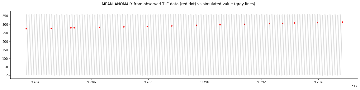
Without knowing what the data is supposed to look like, it is very easy to fit a line across due to the traits that this feature has. To tackle this problem, REV_AT_EPOCH was used and combined with MEAN_ANOMALY into a new feature called REV_MA, which should correctly represent the data’s change over time. However, this does not solve the issue completely, as REV_AT_EPOCH is known to be inaccurate at times, and when the value reaches 100,000, it wraps back to 0. Additional processing was done to separate segments of data points based on their REV_AT_EPOCH values.
Custom Loss Functions
Custom loss functions were explored due to undetected data inconsistencies. For example, when calculating the REV_MA feature, a REV_AT_EPOCH value that’s off by 1 will result in a REV_MA value that is off by 360. With known issues related to REV_AT_EPOCH where 100,000 is represented as 10,000 instead of 0, when rolling over and when multiple ground stations representing inconsistent REV_AT_EPOCH values, a prediction that is correct can potentially have a huge loss due to the incorrect targets. Variants of L1 and L2 loss functions where only the best 75% and 95% predictions were tested. A version of the 75% L2 loss resulted in the best overall accuracy for REV_MA predictions.
Additional DBSCAN Features
In the earlier versions of the Neighboring Pairs Model, the ARG_OF_PERICENTER and RA_OF_ASC_NODE loss was converging quickly but remained very high. Upon inspecting the data which resulted in poor predictions, outliers were spotted in these features. The DBSCAN anomaly detection part of the pipeline was revisited with the addition of these features and ultimately improved the loss by two orders of magnitude.
Hyperparameter tuning, Optimizers, and Schedulers
One of the biggest challenges was a vanishing gradient where a model’s loss would exponentially decay. To address this problem, tuning the learning rate was the first counter action. Different model architectures were then explored: deeper and narrower, shallower and wider, bilinear and ResNet28. After reading Loshchilov & Hutter’s paper “Decoupled Weight Decay Regularization”, different optimizers were tested and mostly settling on AdamW while always circling back to turning other hyperparameters like learning rate and model architecture. Some success was also achieved by using the OneCycle scheduler that increases and then decreases the learning rate over each batch introduced by Smith L. & Topin N. in their 2018 paper “Super-Convergence: Very Fast Training of Neural Networks Using Large Learning Rates”. More details can be seen in Appendix E. Random Model Loss Evaluation.
Configurable/Flexible Model Creation
Because of the frequent experimentation of different model architectures, a convenience method was created that accepts any number of arguments and builds a model based on the name and sequence of the kwargs. This modularity along with using py scripts for the model allowed notebook code to be easier to maintain and reuse the code through different model evolutions. An example of how a model could be created using this approach and the code can be found in Appendix C. Simple Neural Network Investigation.
Model Saving, Loading, and Rollback
When exploring different neural network architectures as well as the choice of loss function and optimizer hyperparameters, there was a need for loading models which were trained in previous sessions, or to roll back current iterations to an earlier epoch when experiments failed. Manually saving and loading files was tedious and prone to human errors, and a system was developed to automatically save the model, epoch and loss history, loss function, and optimizer whenever a new epoch is completed. When the model performance was deemed not satisfactory, an automatic rollback to the previous best version could be triggered. Manual loading to a previous state of the model was also supported by this system. These enhancements allowed for quick iterative tuning of hyperparameters and also prevented loss of progress when the training process encountered errors.
Discussion
When working on the supervised learning part, one thing that surprised us was how accurate the SGP4 baseline appeared to be, knowing that the data seemed noisy and inconsistent. What we had not realized when we selected SGP4 propagation as our baseline was that the TLE format represented mean element values over a period of time, so the value represented at EPOCH is not without errors. We also ignored the fact that TLE and SGP4 were developed together, with SGP4 sacrificing some accuracy at initial EPOCH for better propagation accuracy. Ultimately, we assumed that both our X and y data was a perfect representation of a satellite’s position at initial and target EPOCH, but in reality, due to the SGP4 algorithm, there were invisible errors that were exposed to our models which were not exposed to the SGP4 baseline. With more time and resources, we could use positioning data that are not derived from TLE or SGP4, such as the ILRS dataset to have a more accurate error representation for the baseline and our models.
With the anomaly detection for unsupervised learning, clustering techniques worked better than expected, but there were still some edge cases which the clustering algorithm could not handle properly. Currently, our unsupervised model does not take time into consideration, and while TLE data from Space-Track generally have consistent frequencies and intervals, sometimes there are instances where a satellite would not have any data for an extended period of time. As discussed in the unsupervised learning section, these would become outliers due to a huge delta over time. We explored normalizing the diff values based on the time interval between data points, but the results were not satisfactory. We did not explore further as the results without normalization appeared acceptable, however, with more time and resources, we should be able to eliminate some false positives with proper normalization using time interval differences.
Since some edge cases did outperform the SGP4 propagation, especially as the epoch difference grew, it is plausible that these models might be used to predict satellite positions in cherry-picked situations. However, we find this to be unethical given the overall performance of the models. SGP4 propagation at this point is still more consistent and predictable than our models and using our models could result in significant errors in judgment.
Statement of Work
- Nicholas Miller
- Data split strategy
- Feature Engineering
- Initial neural network models
- Random Pair Model
- Training and Evaluation
- Final Report
- Tim Chen
- Data collection
- Feature Engineering
- Unsupervised learning outlier detection models
- Neighboring Pair Model
- Training and Evaluation
- Final Report
Thank You
We would like to extend a special thank you to the following people who went above and beyond to help us with this project.
Professor Christopher Brooks
Thank you Chris for kindly making available your high computing resources, nellodee, for this project. This proved to be instrumental in handling this massive dataset and for allowing us to run models 24/7 while utilizing ungodly amounts of RAM.
Professor Patrick Seitzer
Thank you Pat for your patience in helping us understand orbital mechanics and providing us with additional reference materials.
Appendix
A. What is a TLE?
A two-line element set (TLE) is a standardized format for describing a satellite’s orbit and trajectory. Below is an example for the International Space Station.
ISS (ZARYA)
1 25544U 98067A   08264.51782528 -.00002182  00000-0 -11606-4 0  2927
2 25544  51.6416 247.4627 0006703 130.5360 325.0288 15.72125391563537
Example TLE for the International Space Station
Source: Wikipedia
A TLE contains 14 fields, from this, only 9 of these are necessary for the SGP4 algorithm. A target EPOCH is also necessary for the SGP4 algorithm to propagate target position and velocity vectors.
- Epoch Year - The year the TLE was calculated
- Epoch Day - The day and fraction of the day the TLE was calculated
- B-star - The drag term or radiation pressure coefficient
- Inclination - Satellite orbit tilt between 0 and 180 degrees
- Right Ascension of the Ascending Node - Ranging from 0 to 360 degrees
- Eccentricity - A measure of how circular the orbit is ranging from 0 to 0.25 for LEO satellites
- Argument of Perigee - The angle from the ascending node ranging from 0 to 360 degrees
- Mean Anomaly - The angular position measured from pericenter if the orbit was circular ranging from 0 to 360 degrees
- Mean Motion - The angular speed necessary to complete one orbit measured in revolutions per day with a minimum of 11.25 for LEO satellites
B. Machine Learning Pipeline
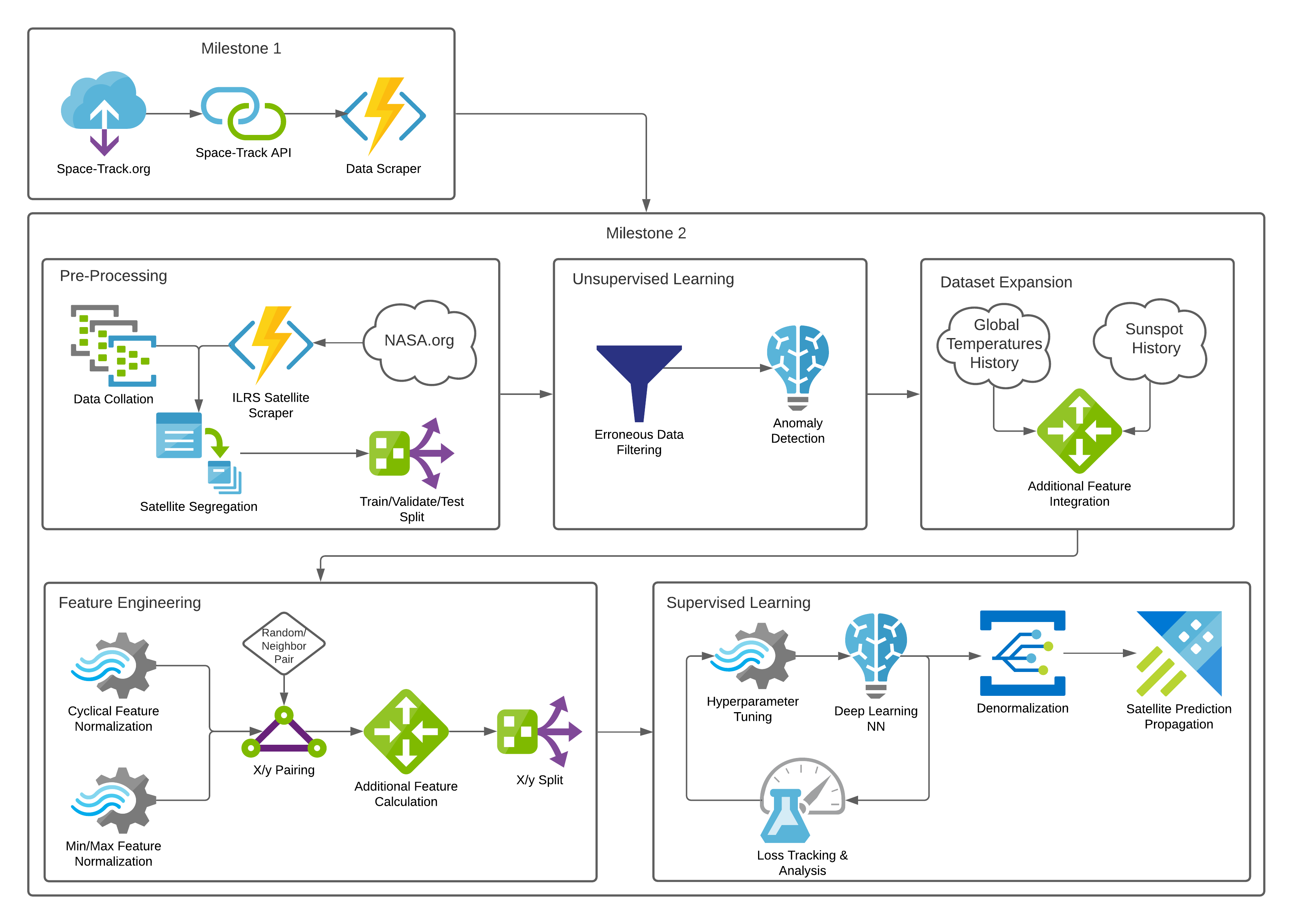
Figure B1 Machine Learning Pipeline
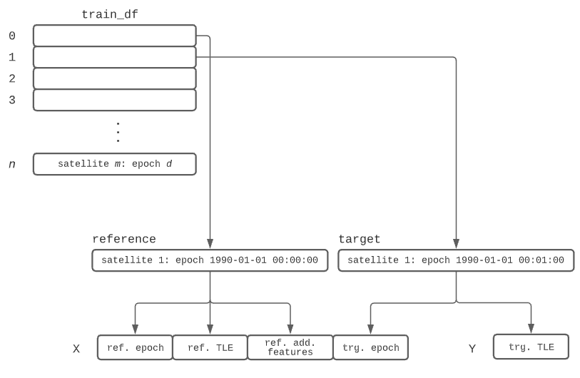
Figure B2 How a X/Y pair was generated
| BSTAR | INCLINATION | RA_OF_ASC_NODE | ECCENTRICITY | ARG_OF_PERICENTER | MEAN_ANOMALY | MEAN_MOTION | |
|---|---|---|---|---|---|---|---|
| 0 | 0.002592 | 62.2415 | 180.1561 | 0.070489 | 265.6761 | 86.2771 | 12.852684 |
| 1 | 0.000100 | 73.3600 | 345.6887 | 0.008815 | 270.3999 | 88.6911 | 12.642166 |
| 2 | 0.001076 | 83.0239 | 250.9465 | 0.008493 | 184.3222 | 175.7249 | 13.856401 |
| 3 | 0.000166 | 70.9841 | 207.4830 | 0.020756 | 161.3777 | 199.5075 | 13.715209 |
| 4 | 0.000739 | 90.1460 | 192.1834 | 0.002746 | 300.4617 | 59.3655 | 12.992417 |
Table B1 Example Raw Y-outputs (not normalized)
C. Simple Neural Network Investigation
| Test L1 Loss | Test L2 Loss | Change History | Time |
|---|---|---|---|
| 0.1234 | 21.7614 | norads=10%, epochs=10, batchSize=200, learn=0.0001, device=cpu, loss=l2, num_workers=5, hidden=300 |
28min 39s |
| 0.1235 | 34.4868 | num_workers=20 | 28min 54s |
| 0.1222 | 30.8207 | norads=20%, num_workers=5 | 53min 47s |
| 0.1219 | 26.2414 | norads=5%, tles-after-1990 | 12min 46s |
| 0.1217 | 0.1226 | remove-high-mean-motion | 13min 22s |
| 0.1211 | 0.1235 | norads=10% | 27min 35s |
| 0.1221 | 0.1232 | hidden=10 | 22min 33s |
| 0.1330 | 0.1380 | updated mean_motion standardization | 24min 16s |
| 0.1329 | 0.1380 | norads=5% | 12min 36s |
| 0.1322 | 0.1385 | run-local | 6min 18s |
| 0.1302 | 0.1373 | num-workers=10 | 4min 44s |
| 0.1302 | 0.1373 | num-workers=10 | 4min 44s |
| 0.1304 | 0.0631 | remove-high-bstar | 4min 37s |
| 0.1289 | 0.0601 | hidden=300 | 8min 31s |
| 0.1423 | 0.0652 | hidden1=100, hidden2=100, drop=50%, batchSize=2000, epoch=5 |
2min 51s |
| 0.1397 | 0.0614 | hidden1=300, drop=50%, hidden2=100, drop=50%, hidden3=10, drop=50%, hidden4=10, drop=50%, hidden5=10, drop=50%, batchSize=2000, epoch=10, learn=0.01 |
6min 12s |
Table C1 Simple Network Change History
For the last few entries, a new model was created that could be initalized with varying number of layers, widths, activation fuctions and dropout:
model = train.create_model(model_cols=model_cols,
                           layer1=300, relu1=True, drop1=0.5,
                           layer2=100, relu2=True, drop2=0.5,
                           layer3=10, relu3=True, drop3=0.5,
                           layer4=10, relu4=True, drop4=0.5,
                           layer5=10, relu5=True, drop5=0.5,
                          )

class NNModelEx(nn.Module):
    def __init__(self, inputSize, outputSize, **kwargs):
        super().__init__()

        network = []
        p = inputSize
        for k,v in kwargs.items():
            if k.startswith('l'):
                network.append(nn.Linear(in_features=p, out_features=v))
                p=v
            elif k.startswith('d'):
                network.append(nn.Dropout(v))
            elif k.startswith('t'):
                network.append(nn.Tanh())
            elif k.startswith('s'):
                network.append(nn.Sigmoid())
            elif k.startswith('r'):
                network.append(nn.ReLU())

        network.append(nn.Linear(in_features=p, out_features=outputSize))
        #network.append(nn.ReLU())

        self.net = nn.Sequential(*network)

    def forward(self, X):
        return self.net(X)
D. Models Learning Data Shape
For the satellite NORAD 10839, the Mean Motion and Right Ascension of the Ascending Node are starting to take shape. This earlier model did not convert some cyclical features resulting in the sawtooth ground truths. Later models converted these features to cyclical features and greatly improved their prediction.
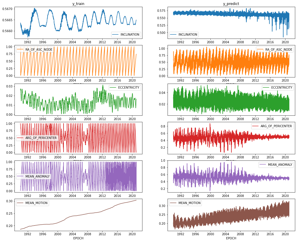
Figure D1 NORAD 10839 Ground Truth and Prediction Comparison
The same can be seen in NORAD 27944.
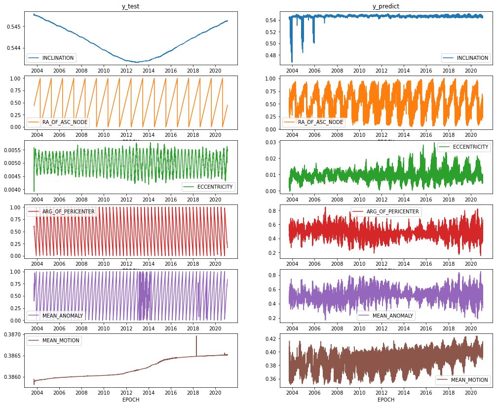
Figure D2 NORAD 27944 Ground Truth and Prediction Comparison
When limiting the models prediction to 14 days and having a separate model for each output feature, the shape of the data is very well preserved as can be seen with NORAD 12701.
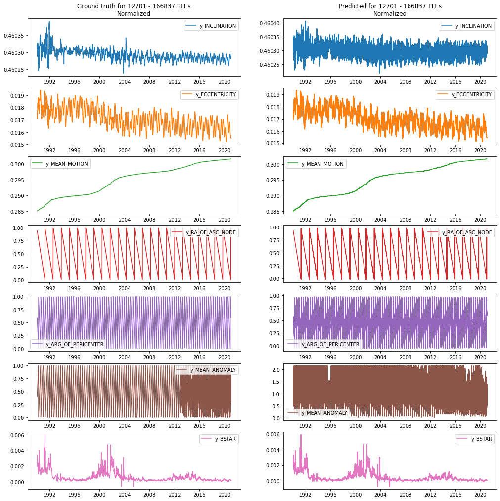
Figure D3 NORAD 12701 Ground Truth and Prediction Comparison (full)
Zooming in on a 1-year period of the previous makes the error more observable.
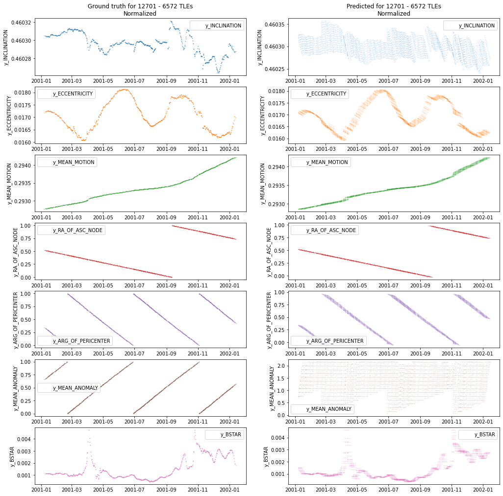
Figure D4 NORAD 12701 Ground Truth and Prediction Comparison (1 Year)
E. Random Model Loss Evaluation
Below is a table showing the optimum loss achieved at 25 epochs for each model evolution.
| v | Model Description | Train Loss 25 Epochs |
Validation Loss 25 Epochs |
|---|---|---|---|
| 1 | 3 fully connected layers width of 100 each hidden layer ReLU between layers |
0.03848 | 0.5963 |
| 2 | ResNet28 (nonlinear regression) width of 256 optimizer Adam |
0.03159 | 0.5297 |
| 3 | ResNet28 (nonlinear regression) width of 256 optimizer AdamW w/ weight_decay=0.00025 |
0.02487 | 1.601 |
| 4 | ResNet28 (nonlinear regression) width of 256 optimizer SGD |
0.03276 | 19.44 |
| 5 | ResNet28 (nonlinear regression) width of 128 (single output) optimizer SGD OneCycle scheduler to epoch 10 then switched to AdamW |
5.176e-06 | 7.604e-07 |
Table E1 random pair variant model evolution
Within each model evolution, hyperparameter tuning took place resulting in various loss trails.
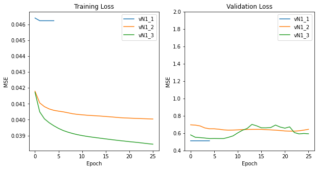
Figure E1 Version 1 First iteration of ResNet28 model
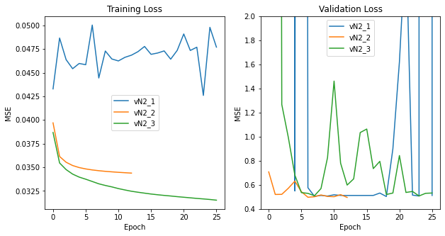
Figure E2 Version 2 Switched from SGD to Adam optimizer
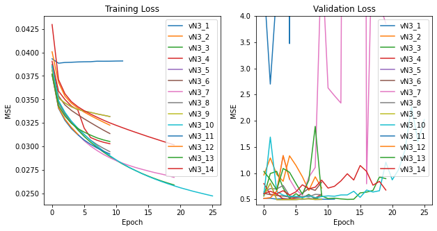
Figure E3 Version 3 Switched from Adam to AdamW optimizer
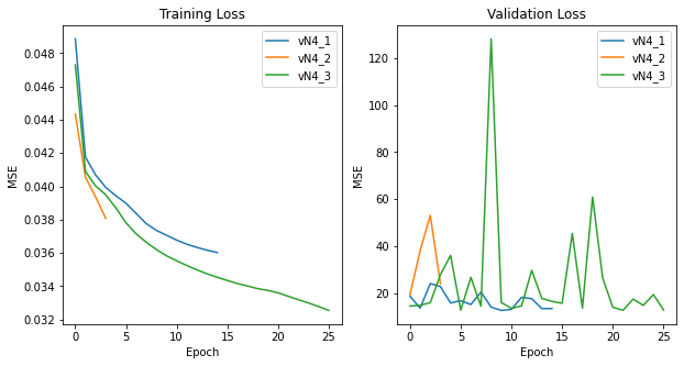
Figure E4 Version 4 Experimented with a "multi-net" model consisting of six
parallel ResNet28 each with a single output.
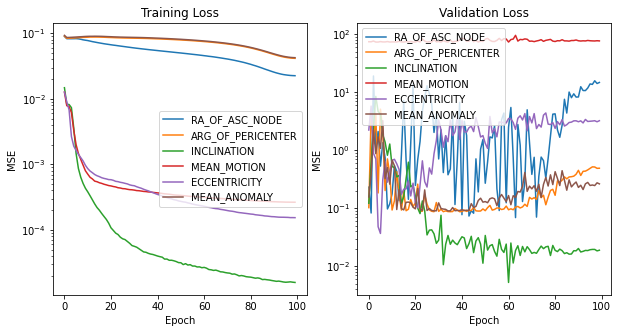
Figure E5 Version 5 Switched to single output models
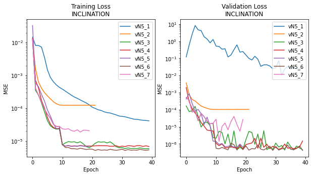
Figure E6 Version 5 Focused on hyperparameter tuning for INCLINATION
F. Anomaly Detection with DBSCAN
Below are the anomaly detection results with the DBSCAN models from selected satellites.
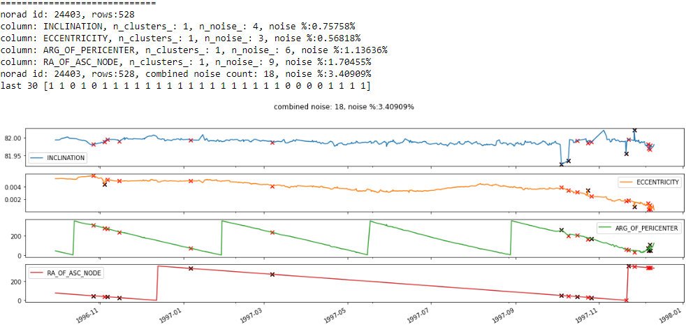
Figure F1 NORAD ID: 24403. PEGASUS DEB (1994-029RG)
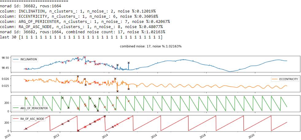
Figure F2 NORAD ID: 36682. FENGYUN 1C DEB (1999-025DZC)
G. Feature Engineering
Below is a table showing details of the features added to the dataset. While all of these features are available, each model may use a different subset of features for training.
| Feature Name | Description | Source | Data Specifications |
|---|---|---|---|
EPOCH_JD |
Julian day representation of EPOCH |
Space-Track TLE | 2447892.5 for 1990-01-01 in increments of 1 per day |
EPOCH_FR |
Remainder of EPOCH_JD, represented as a fraction of a day |
Space-Track TLE | 0-1 |
MEAN_MOTION_DOT |
1st Derivative of the Mean Motion with respect to Time | Space-Track TLE | |
BSTAR |
B* Drag Term, or Radiation Pressure Coefficient | Space-Track TLE | |
INCLINATION |
Orbital inclination measures the tilt of an object’s orbit around a celestial body (degrees) | Space-Track TLE | 0-180 |
RA_OF_ASC_NODE |
Right Ascension of the Ascending Node is the angle measured eastwards (or, as seen from the north, counterclockwise) from the First Point of Aries to the node (degrees) | Space-Track TLE | 0-360 |
ECCENTRICITY |
Eccentricity determines the amount by which its orbit around another body deviates from a perfect circle | Space-Track TLE | 0-0.25 |
ARG_OF_PERICENTER |
Argument of Perigee is the angle from the body’s ascending node to its periapsis, measured in the direction of motion (degrees) | Space-Track TLE | 0-360 |
MEAN_ANOMALY |
The fraction of an elliptical orbit’s period that has elapsed since the orbiting body passed periapsis, expressed as an angle (degrees) | Space-Track TLE | 0-360 |
MEAN_MOTION |
Revolutions per day | Space-Track TLE | Typically 12-16 for satellites in LEO |
SEMIMAJOR_AXIS |
The semi-major axis is the longest semidiameter of an orbit (km) | Space-Track gp_history |
Roughly between 6,400 and 8,400 |
PERIOD |
Orbital period (minutes) | Space-Track gp_history |
84-127 for satellites in LEO |
APOAPSIS |
The largest distances between the satellite and Earth (km) | Space-Track gp_history |
Less than 2,000 for satellites in LEO |
PERIAPSIS |
The smallest distances between the satellite and Earth (km) | Space-Track gp_history |
Less than 2,000 for satellites in LEO |
RCS_SIZE |
Radar cross-section (RCS) size | Space-Track gp_history |
Small, Medium, Large |
EPOCH |
Gregorian datetime representation in UTC | Derived from EPOCH_JD and EPOCH_FR |
|
YEAR |
Gregorian calendar year in UTC | Derived from EPOCH |
1990-2021 |
MONTH |
Gregorian calendar month in UTC | Derived from EPOCH |
1-12 |
DAY |
Gregorian calendar year in UTC | Derived from EPOCH |
1-31 |
HOUR |
Hour of day in UTC | Derived from EPOCH_FR |
0-24 |
MINUTE |
Minute of hour in UTC | Derived from EPOCH_FR |
0-60 |
SECOND |
Second of minute in UTC | Derived from EPOCH_FR |
0-60 |
MICROSECOND |
Microsecond remainder | Derived from EPOCH_FR |
0-1,000,000 |
MEAN_ANOMALY_COS / MEAN_ANOMALY_SIN |
Cartessian representation of MEAN_ANOMALY |
Derived from MEAN_ANOMALY |
-1-1 |
INCLINATION_COS / INCLINATION_SIN |
Cartessian representation of INCLINATION |
Derived from INCLINATION |
-1-1 |
RA_OF_ASC_NODE_COS / RA_OF_ASC_NODE_SIN |
Cartessian representation of RA_OF_ASC_NODE |
Derived from RA_OF_ASC_NODE |
-1-1 |
DAY_OF_YEAR_COS / DAY_OF_YEAR_SIN |
Cyclic transition from last day of the year to first day of the year. | Derived from DAY_OF_YEAR |
-1-1 |
SAT_RX, SAT_RY, SAT_RZ |
Satellite’s x, y, and z coordinates centered around Earth |
Cartesian coordinates by SGP4 | Roughly between -8,000 and 8,000 |
SAT_VX, SAT_VY, SAT_VZ |
Satellite’s x, y, and z vectors |
Cartesian vectors by SGP4 | Roughly between -8 and 8 |
SUNSPOTS_1D, SUNSPOTS_3D, SUNSPOTS_7D |
The rolling average for sunspot count of the past 1, 3, or 7 days. Sunspots are a proxy for solar radiation which has been shown to increase the drag on satellites resulting in faster deorbits. | Sunspot dataset | 0 to 500s |
AIR_MONTH_AVG_TEMP / WATER_MONTH_AVG_TEMP |
Monthly average relative global air and water temperatures. Global warming has shown to lower the density of the upper atmosphere causing decreased satellite drag. | Temperature dataset | -2-+2 |
ARG_OF_PERICENTER_ADJUSTED |
Cumulative ARG_OF_PERICENTER from arbitary 0 |
Derived from a series of ARG_OF_PERICENTER |
|
RA_OF_ASC_NODE_ADJUSTED |
Cumulative RA_OF_ASC_NODE from arbitary 0 |
Derived from a series of ARG_OF_PERICENTER |
|
REV_MEAN_ANOMALY_COMBINED |
Cumulative MEAN_ANOMALY from arbitary 0 |
Derived from a series of MEAN_ANOMALY and REV_AT_EPOCH |
Table G1 Features included or added to dataset
H. Neighboring Pair Model
Generic
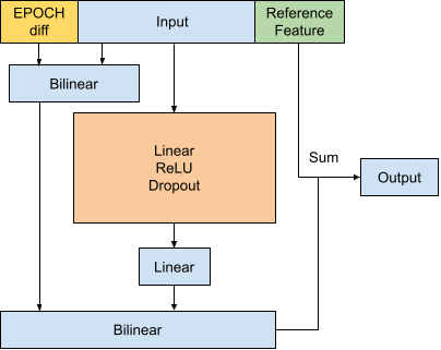
Figure H1 Generic version of Neighboring Pair Model
Mean Anomaly
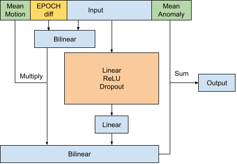
Figure H2 Mean Anomaly version of Neighboring Pair Model
Hidden Layer Configuration (indicated in orange)
| Model | Configuration |
|---|---|
| INCLINATION | 15x100 fully connected layers, ReLU activation, Dropout (50%) |
| ECCENTRICITY | 15x150 fully connected layers, ReLU activation, Dropout (50%) |
| MEAN_MOTION | 4x80 fully connected layers, ReLU activation, Dropout (50%) |
| RA_OF_ASC_NODE | 5x100 fully connected layers, ReLU activation, Dropout (50%) |
| ARG_OF_PERICENTER | 4x300 and 4x150 fully connected layers, ReLU activation, Dropout (50%) |
| MEAN_ANOMALY | 6x60 fully connected layers, ReLU activation, Dropout (40%) |
| BSTAR | 7x60 fully connected layers, ReLU activation, Dropout (50%) |
Table H1 Hidden layer layout
Model Performance and Configurations
| Model | Optimizer (final parameter) | Loss Function | Holdout Loss |
|---|---|---|---|
| INCLINATION | AdamW (lr: 1e-09, weight_decay: 0.057) | MSE | 7.591381967486655e-10 |
| ECCENTRICITY | AdamW (lr: 1e-08, weight_decay: 0.05) | MSE | 3.299049993188419e-07 |
| MEAN_MOTION | AdamW (lr: 1e-08, weight_decay: 0.001) | MSE | 8.657459881687503e-07 |
| RA_OF_ASC_NODE | AdamW (lr: 1e-09, weight_decay: 0.057) | MSE | 2.2815643205831293e-05 |
| ARG_OF_PERICENTER | SGD (lr: 1e-07, momentum: 0.97) | MSE | 0.2577260938386543 |
| MEAN_ANOMALY | AdamW (lr: 1e-07, weight_decay: 0.001) | Custom MAE (top 75%) | 2.5502161747681384e-05 |
| BSTAR | AdamW (lr: 1e-08, weight_decay: 0.001) | MSE | 5.662784955617894e-06 |
Table H2 Model performance
I. Random Pair Model
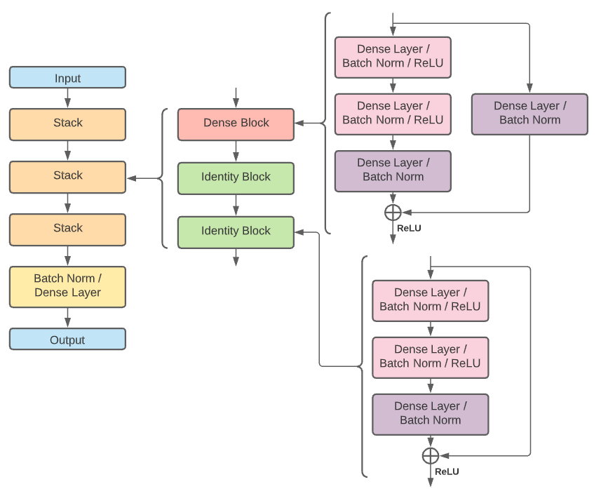
Figure I1 ResNet28 used for Random Pair Model
This model was based on the paper Chen D. et al, 2020 “Deep Residual Learning for Nonlinear Regression”.
J. Mean-Square Error by Epoch Difference
The mean squared error (MSE) for the random model and the neighbor model are shown below when the epoch difference between the reference epoch and the target epoch is normalized and binned. Plotted with the prediction’s MSE is also the X label data MSE (reference TLE values relabeled as output). This was used as a baseline since each TLE’s ground truth values are comparable to the input data.
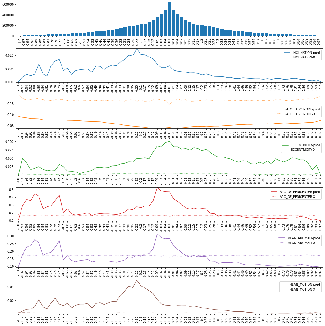
Figure J1 Random Model
In Figure J1, the x-axis ranges from -1 to 1. If a reference TLE epoch was in 2021 and a target epoch was in 1990, the epoch diff would be near 1. If these were flipped, it would be near -1. If the reference and target epochs were within the same year, they would be closer to 0. The top bar chart is a count of records that had an epoch difference in that bin. This model was rather consistent in underperforming against the baseline with the exception being the RA_OF_ASC_NODE.
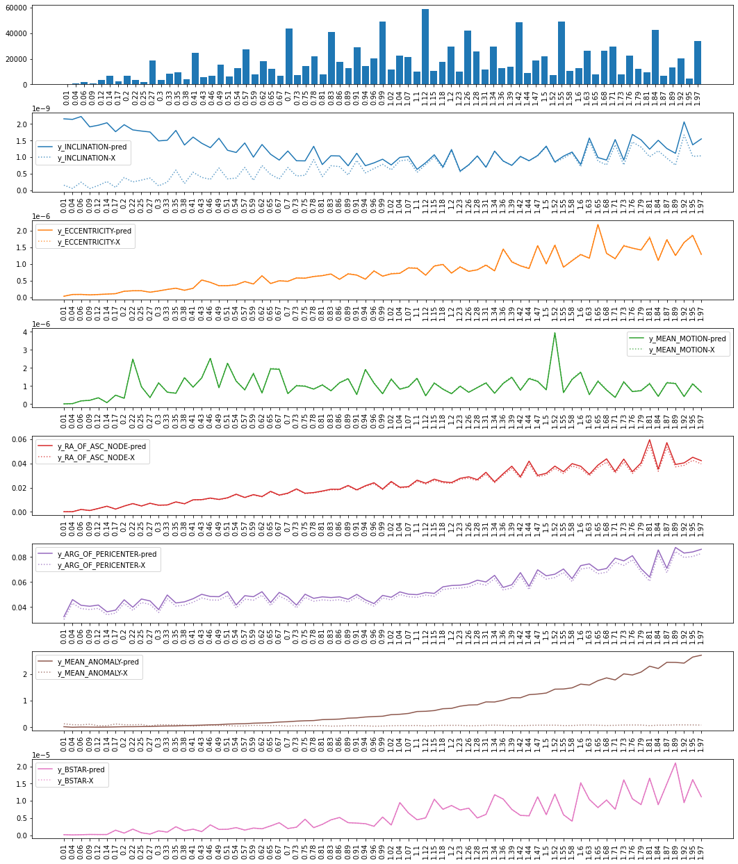
Figure J2 Neighbor Model
In Figure J2, the x-axis ranges from 0 to 2. If a reference TLE epoch was 7 days before a target epoch, the epoch diff would be near 1, hence a difference of 14 days would give a value of 2. If the reference and target epoch were on the same day, they would be closer to 0 This model only trained on future dates so negative values were not possible. The top bar chart is a count of records that had an epoch difference in that bin. This model learned to use the inputs as the outputs.
K. Satellite Position Difference Comparison
Satellites position is calculated by providing a TLE with a reference epoch and a target epoch into the SGP4 algorithm. To create the following graphs, a propagated positions, predicted positions, and ground truth positions were calculated by applying SGP4 on the target epoch to the reference TLE, predicted TLE, and target TLE respectively. Each graph is the straight-line distance between either the propagated postions (from X) or the predicted positions to the ground truth positions.
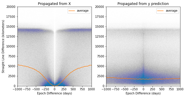
Figure K1 XYZ Difference Random Pair Model (1 model/output)
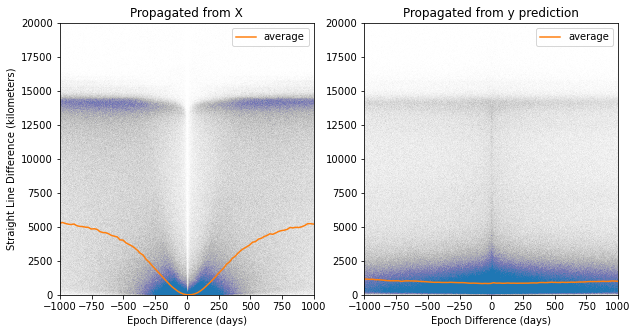
Figure K2 XYZ Difference Random Pair Model (1 model for all outputs)
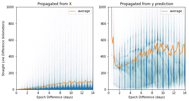
Figure K3 XYZ Difference Neighbor Pair Model
The average lines on the Random Pair Model graphs are the averages on the lower half of the results because some TLEs at these epoch differences create massive errors that skew the average.